
After I found this amazing tutorial on how to visualize any rates on country maps, I desperately wanted to try it.
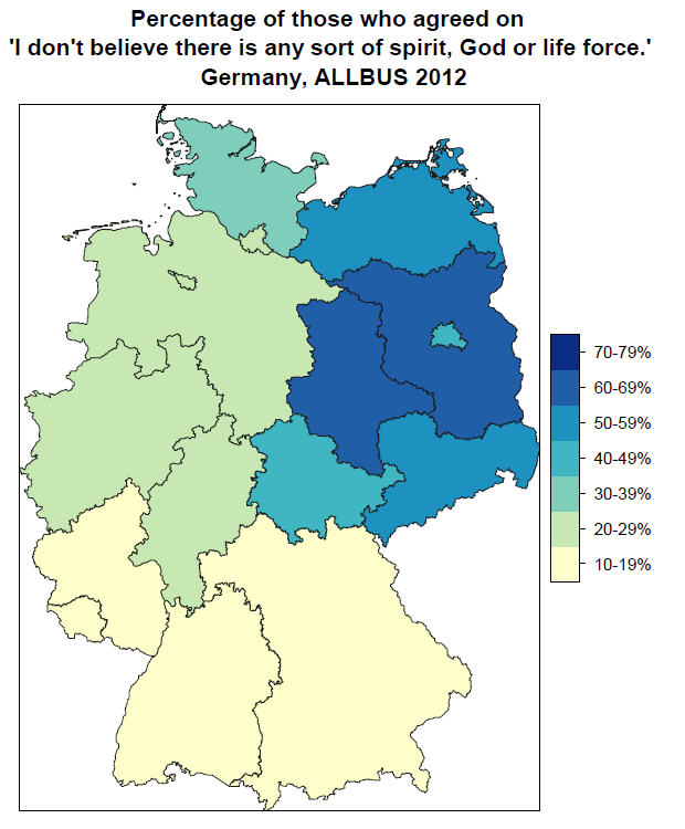
Because it’s useless to visualize things just to make pretty colourful maps, I decided to overcome this map’s shortcomings. When asked which statement represents them best, respondents could chose between “I believe in a personal god”, “I believe there is some sort of spirit or life force” or “I don’t believe there is any sort of spirit, God or life force”. Aggregation on the national level makes it look like around 35% of all Germans don’t believe in any sort of God or higher spirit.
When it comes to religion (among of other cultural things), it’s always important to treat East and West Germany separately, you’ll immediately see why.
As far as I know, the latest data available to analyze this for Germany is the ALLBUS 2012. Sadly, no information was available below Länder level. I used Stata to calculate the means and spatial data for Germany from the gadm.
I’m not that satisfied with it because I don’t like the font that much and it could look a bit more polished (and I wasn’t able to include text with the source information). But I really liked the process of doing it, so I’m doing that for Europe next on the NUTS2-level. I’m jealous of all Geography students though that seem to learn that as part of their coursework. But it’s a nice opportunity to get back to R.
So how to do this?
This is how it worked for me. It’s not the most elegant or parsimonious code for sure, but it leads to results.
You need three things:
A purpose, the spatial data and the data rates for the single entities. In this example, I use the rates for atheism per German state.
## First step: Load the spatial data
## get spatial data for Germany on state level, change to DEU_adm2 for Regierungsbezirke and DEU_adm3 for cities and Kreise
con <- url("http://gadm.org/data/rda/DEU_adm1.RData")

print(load(con))

close(con)
## plot Germany with random colors
col = rainbow(length(levels(gadm$NAME_1)))

spplot(gadm, "NAME_1", col.regions=col, main="German Regions",

colorkey = FALSE, lwd=.4, col="white")
## Second step: Load the information for the entities that you calculated with the software of your choice stored in a .txt or .csv-file seperated by tabs or ; etc
## Allbus does distinguish between Berlin-East and Berlin-West so I had to merge those two before I calculated the rates per state
## In this example, the first column contains the entity names (here the state names), the second column the rates. Headers are “Land” and “Rates”
# dec=”.” can be changed to dec=”,” if your data has “,” as decimal separators; if your file is comma-separted change “sep=”\t” accordingly
nobeliever<- read.delim2(file="allbus2012_dontbelieveingod.txt", header = TRUE, sep = "\t",

dec=".", stringsAsFactors=F)
## Now you have to data frames, gadm and nobeliever,
## Third step: Merge both frames
## First, you need to bring gadm and the nobeliever data frames into the same order to match them later,
## I use the code from http://ryouready.wordpress.com/2009/11/16/infomaps-using-r-visualizing-german-unemployment-rates-by-color-on-a-map/
## That might take some time
total <- length(gadm$NAME_1)

order <- vector()

for (i in 1:total){

order[i] <- agrep(gadm$NAME_1[i], nobeliever$Land,

max.distance = 0.2)[1]

}
## 1 Cut into intervals
## You need to cut your values into intervals, so check your rates and chose the intervals, assign their level names.
nobeliever[order(nobeliever$Rate),]
##I chose to divide them into decentiles. As no state has a rate below 10, the intervall 0-9% would be empty, so no need to include it
col_no <- as.factor(as.numeric(cut(nobeliever$Rate[order],

c(0.10,0.19,0.29,0.39,0.49,0.59,0.69))))

levels(col_no) <- c("10-19%","20-29%", "30-39%", "40-49%", "50-59%", "60-69%")
## Assign col_no to the gadm data frame
gadm$col_no <- col_no
## Check how many levels you’ve got
col_no
## 2 Choose the colours
## The number of the colours must match the number of levels
## Use RColorBrewer to obtain different colors for the amount of levels you have. #f one of your intervals is empty, you will get an error
## display.brewer.all() shows you all available choices
myPalette<-brewer.pal(6,"YlGnBu")
## 3 Draw the map
## col=grey(.4) changes the borders
spplot(gadm, "col_no", col=grey(.4), col.regions=myPalette,

main="Percentage of those who agreed on \n'I don't believe there is any sort of spirit, God or life force.'\n Germany, ALLBUS 2012")
Just save this in a text-File.
Land Rate
Baden-Württemberg 0.1446384
Bayern 0.1550562
Berlin 0.4
Thüringen 0.452514
Brandenburg 0.6052632
Bremen 0.25
Hamburg 0.25
Hessen 0.221374
Mecklenburg-Vorpommern 0.572327
Niedersachsen 0.2364865
Nordrhein-Westfalen 0.2190305
Rheinland-Pfalz 0.1761006
Saarland 0.1818182
Sachsen 0.5166667
Sachsen-Anhalt 0.6300578
Schleswig-Holstein 0.36
